Tutorial 3: Regression modelling in R
Aims
By the end of this third tutorial, you will be able to
- fit regression models in R.
- interpret linear models in context.
- understand the uncertainty in model predictions.
Linear regression modelling - an example
A common use of linear regression models is to predict quantities that are are otherwise difficult or expensive to measure directly. One example is predicting a person’s percentage body fat. This is clinically useful information, because it is a good indicator of some disease outcomes.
But body fat percentage is not easy to measure precisely. A commonly used precise method relies on the fact that muscle and bone are both denser than fat. By submerging an individual in water, we can obtain a measure of their body’s volume. Knowing this and their weight, we can compute their average density, $d$, in $g/cm^3$ . Previous studies (Brozek 1963) have shown that the percentage of body fat is then given approximately by the formula
\[\left(\frac{4.57}{d} − 4.142\right) × 100\%,\]to within a precision of around $1\%$ , which is good enough.
The data
We’ll work with the fat dataset from the faraway package (Faraway
2004). You will need to install this package if you have not used it
before, using install.packages("faraway"). Once the package is
installed, it must be loaded,
library(faraway)
The help file ?fat gives some useful background information on the
data we’ll be using. The data consists of 10 body circumference
measurements for 252 men, together with information on their age, weight
and height.
In addition, each individual’s density was measured by submerging them in water, and their percentage body fat was estimated precisely using Brozek’s equation (Johnson 1996).
Exploratory data analysis
To familiarise yourself with the structure of the data, enter the
command View(fat) in the console to get a spreadsheet representation
of the data.
Matching up the names of the variables with the information in the help file, we see that the first two columns give estimates of the body fat percentage using Brozek’s equation and another method, Siri’s equation. We then have density, age, weight, height and adiposity (more commonly known as BMI - body mass index).
As a simple check that we understand the data, we make a plot of
brozek against density. The data points should all lie on a smooth
curve.
plot(fat$density, fat$brozek)
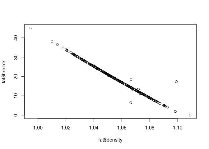
Almost all of the observations do lie on a smooth curve, but there are some unusual observations that might be a cause for concern.
To make the relationship even clearer, we could apply the Brozek equation ourselves, and compare the result with that in the data.
plot(457/fat$density - 414.2, fat$brozek)
abline(0, 1, col = "red")
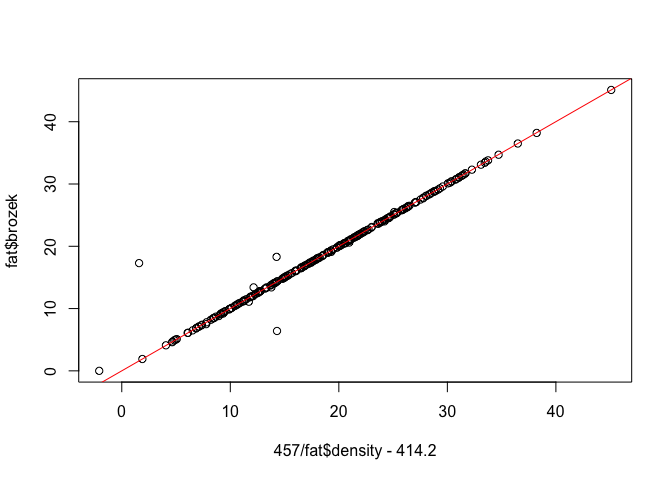
The red line is $y = x$ , showing that apart from a few outlying observations, the density and Brozek values match up well.
Now we look at the body circumference measurements, stored in columns 9 to 18 of the data frame.
One way to visualise how the measurements are distributed is to look at a pairs plot. For each pair of variables, we make a scatter plot. They can be seen in the plot below.
library(GGally)
ggpairs(fat[,9:18],
        upper = list(continuous = wrap("cor", size = 3)))
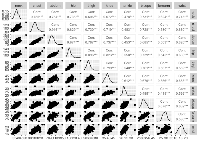
Note the roughly elliptical shape visible in the plot of each pair of variables, aligned on the diagonal.
This suggests two observations
-
The data are jointly normally distributed. This is what we would expect for naturally occurring data, influenced by many genetic and environmental factors.
-
Pairs of variables are strongly positively correlated. This makes sense: on average, individuals with larger necks will have larger knees, forearms etc.
Linear modelling
Focusing for now on a single variable, we make a plot of the Brozek fat estimate against chest circumference.
plot(fat$chest,
     fat$brozek,
     xlab = "chest circumference (cm)",
     ylab = "% body fat")
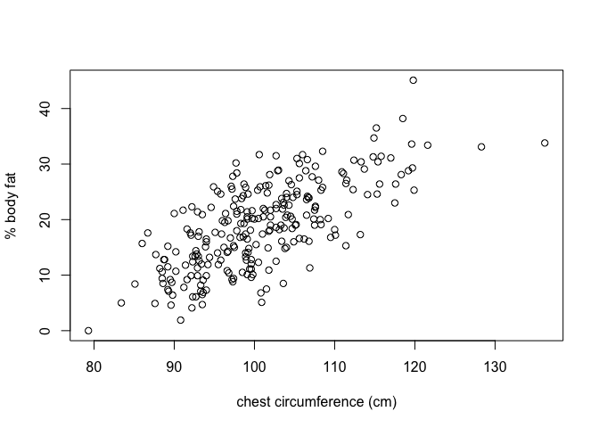
There is clearly a linear relationship between the two quantities,
although it is somewhat noisy. We determine the equation of the best
fitting line representing this relationship using the lm command (it
stands for linear model).
Note the syntax used for fitting the model: brozek ~ chest. We say
this out loud as Brozek is explained by chest.
fit0 = lm(brozek ~ chest, data = fat)
More explicitly, the model is \(\text{brozek}_i =\beta_0 +\beta_1\text{chest}_i +\epsilon_i,\)
where $\text{brozek}_i$ and $\text{chest}_i$ represent the Brozek body fat estimate and chest circumference of individual $i$, $\beta_0$ and $\beta_1$ are the y-intercept and slope of the line and $\epsilon_i$ is a random error.
Model fitting
The lm function determines good values of the model parameters $\beta_0$ and $\beta_1$
, in the sense of minimising a measure of the average error when using
the line to make predictions.
A more mathematically complete account of how regression works can be found in the supplementary tutorial.
The model summary contains a wealth of information about the linear
model that lm has determined.
summary(fit0)
##
## Call:
## lm(formula = brozek ~ chest, data = fat)
##
## Residuals:
##      Min       1Q   Median       3Q      Max
## -13.8875  -3.8211  -0.2752   3.4950  13.8989
##
## Coefficients:
##              Estimate Std. Error t value Pr(>|t|)
## (Intercept) -46.21636    4.18460  -11.04   <2e-16 ***
## chest         0.64622    0.04136   15.62   <2e-16 ***
## ---
## Signif. codes:  0 '***' 0.001 '**' 0.01 '*' 0.05 '.' 0.1 ' ' 1
##
## Residual standard error: 5.524 on 250 degrees of freedom
## Multiple R-squared:  0.494,  Adjusted R-squared:  0.492
## F-statistic: 244.1 on 1 and 250 DF,  p-value: < 2.2e-16
There is a lot to make sense of here. We’ll start by identifying the
most important values in the coefficient table. Here we see the
estimate of the intercept -46.21636 and the estimate of the slope
0.64622.
This says that the best-fitting line is given by
\[\text{brozek}_i = -46.21636 + 0.64622\times\text{chest}_i.\]We can add this line to our earlier plot,
plot(fat$chest,
     fat$brozek,
     xlab = "chest circumference (cm)",
     ylab = "% body fat")
abline(fit0, col = "red")
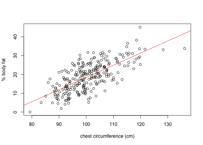
Showing a reasonable fit to the data.
Parameter uncertainty
The second column of the coefficient table gives the standard error of each parameter estimate. This is a measure of the uncertainty in the estimate that comes from having used only a fairly small sample: slightly different data would of course have led to slightly different estimates.
We see that the standard error of the slope estimate is 0.04136. What
this number tells us is that the slope estimate of 0.64622 is only
really correct to one significant figure. If we had chosen different
samples from the population, we could very easily have estimated the
slope as anywhere in the interval $0.64\pm 0.04$
.
Interpreting model parameters
Note the units of the parameters we have estimated. The intercept
parameter has the same units as brozek, i.e. percentage body fat, and
the slope has units of percentage body fat per centimetre of chest
circumference.
The interpretation of the slope parameter is that, all other things being equal, each additional centimetre of chest circumference is associated with an increase in body fat of $\sim 0.6$ percentage points.
Residual standard error
The model summary shows a residual standard error of 5.524. This
is a measure of the typical variability around the line, in the
vertical direction. Its units are percentage body fat. It is a measure
of how precise predictions from the model are expected to be: our
predicted body fat percentages would only be correct to around 5.5
percentage points - considering the range of the data, this is not
really an adequate level of precision. Someone with 20% body fat might
easily be estimated as having 15% body fat or 25% body fat.
Improving the model
We can improve the fit of the model by including all of the other variables as additional predictors.
fit1 = lm(brozek ~ age + weight + height +
             neck + chest + abdom +
             hip + thigh + knee +
             ankle + biceps + forearm + wrist,
           data = fat)
summary(fit1)
##
## Call:
## lm(formula = brozek ~ age + weight + height + neck + chest +
##     abdom + hip + thigh + knee + ankle + biceps + forearm + wrist,
##     data = fat)
##
## Residuals:
##     Min      1Q  Median      3Q     Max
## -10.264  -2.572  -0.097   2.898   9.327
##
## Coefficients:
##              Estimate Std. Error t value Pr(>|t|)
## (Intercept) -15.29255   16.06992  -0.952  0.34225
## age           0.05679    0.02996   1.895  0.05929.
## weight       -0.08031    0.04958  -1.620  0.10660
## height       -0.06460    0.08893  -0.726  0.46830
## neck         -0.43754    0.21533  -2.032  0.04327 *
## chest        -0.02360    0.09184  -0.257  0.79740
## abdom         0.88543    0.08008  11.057  < 2e-16 ***
## hip          -0.19842    0.13516  -1.468  0.14341
## thigh         0.23190    0.13372   1.734  0.08418.
## knee         -0.01168    0.22414  -0.052  0.95850
## ankle         0.16354    0.20514   0.797  0.42614
## biceps        0.15280    0.15851   0.964  0.33605
## forearm       0.43049    0.18445   2.334  0.02044 *
## wrist        -1.47654    0.49552  -2.980  0.00318 **
## ---
## Signif. codes:  0 '***' 0.001 '**' 0.01 '*' 0.05 '.' 0.1 ' ' 1
##
## Residual standard error: 3.988 on 238 degrees of freedom
## Multiple R-squared:  0.749,  Adjusted R-squared:  0.7353
## F-statistic: 54.63 on 13 and 238 DF,  p-value: < 2.2e-16
Inspecting the summary, we see that the residual standard error has
reduced to 3.988, an improvement, although still a little too
imprecise for clinical use.
Here, adding further predictors did not really lead to a substantial improvement in the model’s predictions. The main reason for this is that the predictors we added are highly correlated: they are not independent sources of information.
Including highly correlated predictors in this way is not advisable - it
means that individual parameters are estimated less precisely. We can
see that in fit1, the standard error of our original predictor,
chest has increased to 0.09.
Conclusion
These tutorials have guided you through some first steps in learning R. You are now well-equipped to explore data independently in R and to fit regression models.