Tutorial 1: First Steps with R
These tutorials provide a self-contained introduction to the R language, a powerful and widely-used environment for working with data.
Aims
By the end of this first tutorial, you will be able to
- work confidently in the R console.
- define and manipulate variables
- make simple graphics.
Installation
You can obtain a free copy of R from www.r-project.org. Install files are available for Windows, Mac and Linux.
In this tutorial, we will use RStudio, a nicely designed interface for working with the R language. It can be freely downloaded from rstudio.com
The R console
When you first open RStudio, you will see an environment with several windows.
The console is where commands are entered. By default, it will appear bottom left. The console will be our main way of interacting with R. Type the following three commands into the console, one at a time. Check that the output is what you expect.
2+3
4^2
sin(pi/2)
R stores data as objects. At its simplest, we can store a value in an object using the following syntax
x = 4
Type the command above into the console, noting any changes in the Environment tab in the top right of the RStudio window.
A common alternative way to assign objects in R is
x <- 4
This works just as well. But it is quite peculiar for those who are used to other languages.
To access the contents of a variable, enter its name in the console.
x
Variables containing numeric values can be manipulated as numbers. Check that the commands below behave as you expect.
x + x
3 * x
x ^ 2
sqrt(x)
x / x
A variable can be removed using the command rm.
rm( x )
Arrays
Typically, we want to work with data sets that contain many values. In R, data are stored as arrays. Most simply, we have vectors that are defined as follows.
a = c( 1, -2.3, 4.5, 9, 150 )
c stands for combine.
Functions
Properties of a variable can be extracted with a function, e.g.
length(a)
returns the length of the vector a.
Help
Any built-in R function comes with an extensive help file
?length
The help file explains how to use the function. It will always contain a working example that you can adapt.
Subsetting
We often need to access particular entries of a vector. Try to understand what the following commands achieve.
a[3]
a[c(2, 4)]
a[c(2 : 4)]
a[-3]
a[-c(1, 2)]
Working with data
As a first example, we will use the iris dataset, which is supplied
with R. Background information is available from the help
?iris
First, we display the data as a rectangular array, which will appear in a separate window. There are 150 observations, and five different variables. An observation corresponds to a row, and a variable corresponds to a column.
View(iris)
Four of the variables are numerical, and one, species, is categorical.
We can extract entries from the array as follows.
To obtain the values for the first observation, we extract the first row
iris[ 1 ,]
##   Sepal.Length Sepal.Width Petal.Length Petal.Width Species
## 1          5.1         3.5          1.4         0.2  setosa
To obtain the values for the first variable, we extract the first column
iris[ , 1 ]
##   [1] 5.1 4.9 4.7 4.6 5.0 5.4 4.6 5.0 4.4 4.9 5.4 4.8 4.8 4.3 5.8 5.7 5.4 5.1
##  [19] 5.7 5.1 5.4 5.1 4.6 5.1 4.8 5.0 5.0 5.2 5.2 4.7 4.8 5.4 5.2 5.5 4.9 5.0
##  [37] 5.5 4.9 4.4 5.1 5.0 4.5 4.4 5.0 5.1 4.8 5.1 4.6 5.3 5.0 7.0 6.4 6.9 5.5
##  [55] 6.5 5.7 6.3 4.9 6.6 5.2 5.0 5.9 6.0 6.1 5.6 6.7 5.6 5.8 6.2 5.6 5.9 6.1
##  [73] 6.3 6.1 6.4 6.6 6.8 6.7 6.0 5.7 5.5 5.5 5.8 6.0 5.4 6.0 6.7 6.3 5.6 5.5
##  [91] 5.5 6.1 5.8 5.0 5.6 5.7 5.7 6.2 5.1 5.7 6.3 5.8 7.1 6.3 6.5 7.6 4.9 7.3
## [109] 6.7 7.2 6.5 6.4 6.8 5.7 5.8 6.4 6.5 7.7 7.7 6.0 6.9 5.6 7.7 6.3 6.7 7.2
## [127] 6.2 6.1 6.4 7.2 7.4 7.9 6.4 6.3 6.1 7.7 6.3 6.4 6.0 6.9 6.7 6.9 5.8 6.8
## [145] 6.7 6.7 6.3 6.5 6.2 5.9
Note that we can also refer to the variables by their names
iris$Sepal.Length
##   [1] 5.1 4.9 4.7 4.6 5.0 5.4 4.6 5.0 4.4 4.9 5.4 4.8 4.8 4.3 5.8 5.7 5.4 5.1
##  [19] 5.7 5.1 5.4 5.1 4.6 5.1 4.8 5.0 5.0 5.2 5.2 4.7 4.8 5.4 5.2 5.5 4.9 5.0
##  [37] 5.5 4.9 4.4 5.1 5.0 4.5 4.4 5.0 5.1 4.8 5.1 4.6 5.3 5.0 7.0 6.4 6.9 5.5
##  [55] 6.5 5.7 6.3 4.9 6.6 5.2 5.0 5.9 6.0 6.1 5.6 6.7 5.6 5.8 6.2 5.6 5.9 6.1
##  [73] 6.3 6.1 6.4 6.6 6.8 6.7 6.0 5.7 5.5 5.5 5.8 6.0 5.4 6.0 6.7 6.3 5.6 5.5
##  [91] 5.5 6.1 5.8 5.0 5.6 5.7 5.7 6.2 5.1 5.7 6.3 5.8 7.1 6.3 6.5 7.6 4.9 7.3
## [109] 6.7 7.2 6.5 6.4 6.8 5.7 5.8 6.4 6.5 7.7 7.7 6.0 6.9 5.6 7.7 6.3 6.7 7.2
## [127] 6.2 6.1 6.4 7.2 7.4 7.9 6.4 6.3 6.1 7.7 6.3 6.4 6.0 6.9 6.7 6.9 5.8 6.8
## [145] 6.7 6.7 6.3 6.5 6.2 5.9
R makes it easy to make simple graphics to visualize relationships in data. As a simple example, let’s look at the relationship between the length and width of iris petals
plot(iris$Petal.Length, iris$Petal.Width )
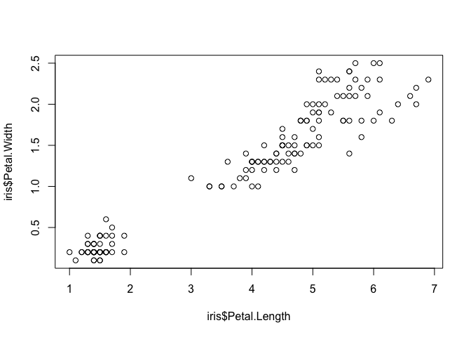
Note the (entirely expected) positive correlation between the two variables.
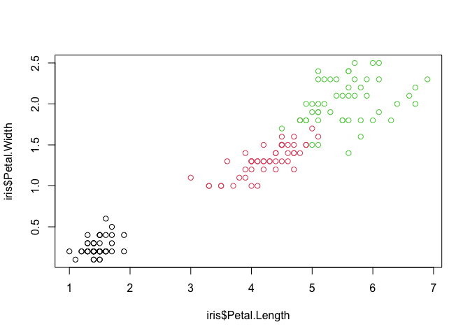
We can add more information by colouring the points according to the
species variable. To make the code easier to read, the arguments to
the function appear on separate lines.
plot(iris$Petal.Length,
     iris$Petal.Width,
     col = iris$Species)
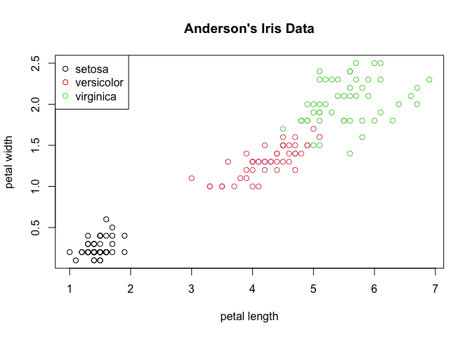
Finally, let’s smarten up the plot by adding labels and a legend.
plot(iris$Petal.Length,
     iris$Petal.Width,
     col = iris$Species,
     main = "Anderson's Iris Data",
     xlab = "petal length",
     ylab = "petal width")

legend("topleft",
       legend=c("setosa","versicolor","virginica"),
       col=c("black", "red","green"),
       pch=1)
Packages
You will need to install packages to make some functions in these
tutorials work. For instance, we install the common graphics library
ggplot2 as follows
install.packages("ggplot2")
Note the quotation marks.
This only needs to be done once. Whenever the package is used in a new session, it must be loaded using the command
library(ggplot2)
Next steps
In the next tutorial, we will work with some data. After completing this tutorial, you will be able to
- load in data.
- make exploratory graphics.
- perform elementary manipulations on a data frame.