Tutorial 2: Working with data in R
Aims
By the end of this second tutorial, you will be able to
- Import data files into an R data frame
- Make exploratory graphics
- Perform elementary manipulations on a data frame.
Downloading and importing data
In R it is straightforward to import data that are stored locally on your machine or directly from the web. We’ll import some data from Our World In Data. You can access the data from the data file directly here. The variables are explained in the code book.
Within RStudio, there is a neat interface for reading in data. In the
Environment tab in the top right corner of the RStudio window,
select Import Dataset and From Text (readr)…. Note that other
options support importing data in Excel and other common formats. Some
of the functionality here is from the tidyverse suite of packages, a
widely used framework for Data Science in R.
In the dialog box that opens, navigate to the folder where the downloaded file is located. Once you have selected the file, the window will show a preview of how the data will be imported. For this dataset, the data should appear as a neat, rectangular array. This means we are now ready to import the data. Other datasets might require more effort.
The Code Preview box gives a few lines of code that could be used to read in the data manually. Instead, simply click Import. Then R runs the code from the Code Preview box.
Alternatively, we could read in the file directly from the web. To do
this, we need to load the tidyverse.
library(tidyverse)
dat_url = "https://nyc3.digitaloceanspaces.com/owid-public/data/energy/owid-energy-data.csv"
dat = read_csv(dat_url)
Exploring data
The View(dat) command produces a nice interactive spreadsheet
representation of the data, which appears in a separate panel. There are
many different variables - look through the codebook to understand what
each variable means.
We’ll now see some tools for exploring the data and constructing some simple plots.
First, we’ll restrict our attention to the data relating to the United Kingdom. We define a new object by filtering the original data object.
dat_uk = filter(dat,
                country == "United Kingdom")
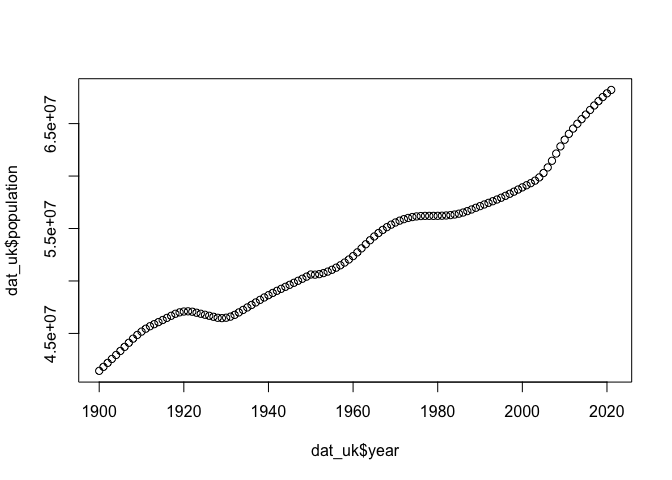
We can make a simple plot of how the UK population has changed over the
time period recorded in the dataset. Note that we use $ to refer to
the columns of our data.
plot(dat_uk$year,
     dat_uk$population)
For this data, perhaps it is more natural to plot a line than to plot
individual points. We can do this by setting the type argument.
plot(dat_uk$year,
     dat_uk$population,
     type = "l")
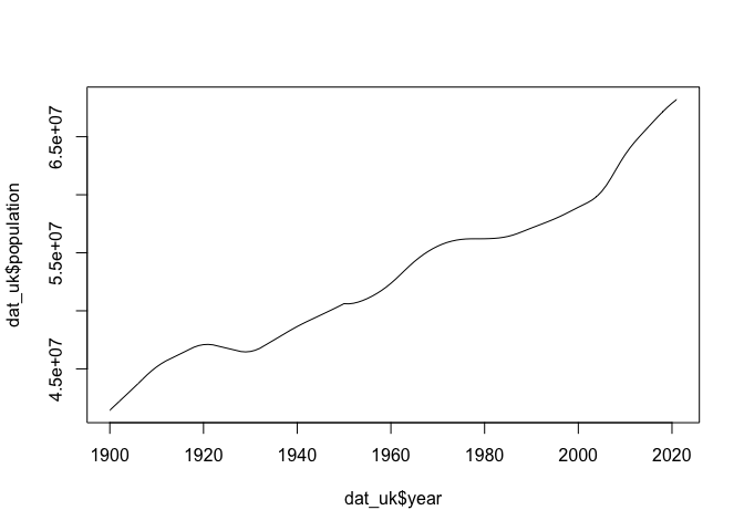
This is better, although there is still more work to do before we have a plot that we would be happy including in a well-presented report.
ggplot for data-controlled graphics
The ggplot package allows very precise control of how plots are made.
It is especially useful when working with large, structured datasets.
The gg in`ggplot refers to the Grammar of Graphics, a framework
for specifying precisely how elements of a data visualisation are built
up on the page.
The syntax takes some getting used to. We’ll start by giving the full command, and then breaking it down.
ggplot( dat = dat_uk,
        mapping = aes(x = year,
                      y = population)) +
  geom_line()
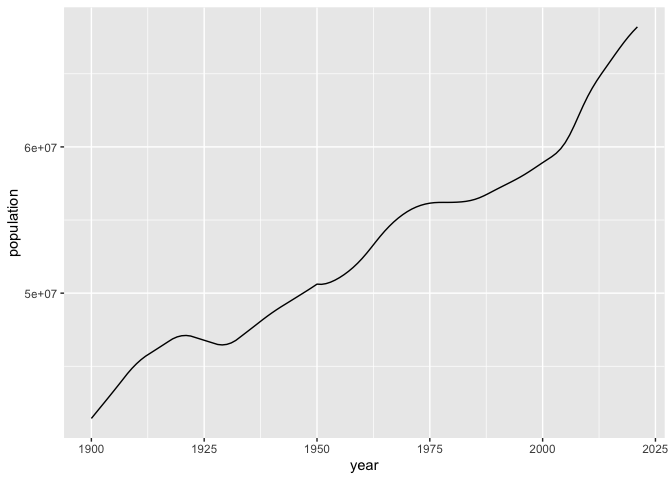
The first argument is the data frame to be used for plotting: here, this
is dat_uk. We then specify a mapping. This determines how variables
in the dataset correspond to visual properties. Here, we specify that
the x-axis is controlled by the year variable, and the y-axis by the
population variable.
The term after the + specifies a new layer to be placed on the
plotting environment. In this case, we specify a line.
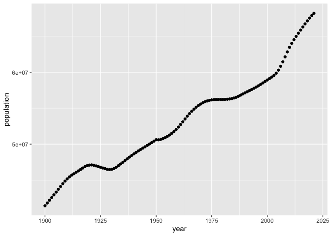
We could alternatively plot individual data points.
ggplot( dat = dat_uk,
        mapping = aes(x = year,
                      y = population)) +
  geom_point()
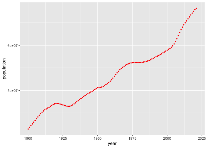
We can control properties of the plotted points by specifying the
appropriate aesthetics. You can obtain a full list of the properties
from the help ?geom_point under aesthetics. Here we change the
colour and size.
ggplot( dat = dat_uk,
        mapping = aes(x = year,
                      y = population)) +
  geom_point(colour = "red",
             size = 0.75)
One very useful feature of ggplot is the ability to modify the
properties of points (or lines) using values in the data.
As a simple example, we define an indicator variable, which is TRUE if
the year is later than 1975, and FALSE otherwise.
dat_uk$indicator = dat_uk$year > 1975
We then pass the indicator variable to geom_point as an aesthetic
controlling the colour.
ggplot( dat = dat_uk,
        mapping = aes(x = year,
                      y = population)) +
  geom_point(aes(colour = indicator))
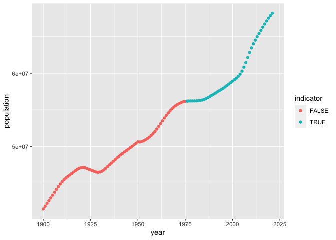
Now points are coloured differently according to whether or not they are later than 1975.
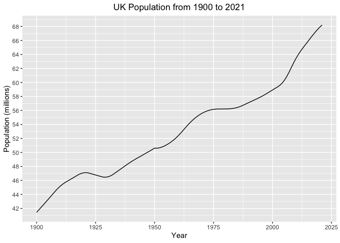
Modifying plot attributes
We’ll now make the plot easier to read. We make the following changes
-
Measure population in units of millions, by dividing the population variable by $10^6$ .
-
Add neat labels for the x- and y-axes, and a centred title.
-
Change the y-axis scale so that tick marks occur at evenly spaced values between 40 and 70.
ggplot( dat = dat_uk,
        mapping = aes(x = year,
                      y = population/10^6)) +
  geom_line() +
  scale_x_continuous("Year") +
  scale_y_continuous("Population (millions)",
                     breaks = seq(40, 70, 2)) +
  ggtitle( "UK Population from 1900 to 2021") +
  theme(plot.title = element_text(hjust = 0.5))
Comparing countries
Let’s now add data from some other countries to the plot. So that the plot isn’t too busy, we will just consider a few countries, with broadly similar populations.
Start by making a new data frame.
dat_small = filter(dat, country %in%
                          c("United Kingdom",
                            "France",
                            "Germany",
                            "Spain"))
Then plot, specifying in the aesthetic that colour is controlled by
the variable country.
ggplot( dat = dat_small,
        mapping = aes(x = year,
                      y = population/10^6,
                      colour = country)) +
  geom_line() +
  scale_x_continuous("Year") +
  scale_y_continuous("Population (millions)",
                     breaks = seq(20, 100, 5)) +
  ggtitle( "UK Population from 1900 to 2021") +
  theme(plot.title = element_text(hjust = 0.5)) +
  labs(colour = "Country")
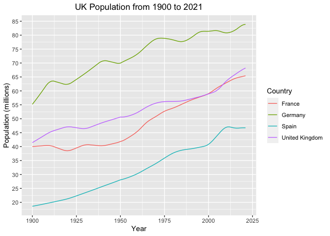
Note two additional changes in the plot above: to the range of y-axis
values, to account for the wider range of values, and to the
specification of the legend label in the final labs argument.
Manipulating data frames
The two most important functions for manipulating data frames are
filter and select. We have already seen that filter extracts
observations (rows of the data frame). select extracts variables
(columns of the data frame).
e.g. if we wanted to extract all variables relating to coal, we could use the following code
select(dat, contains("coal"))
## # A tibble: 22,343 × 12
##    coal_cons_change_pct coal_cons_change_twh coal_cons_per_cap… coal_consumption
##                   <dbl>                <dbl>              <dbl>            <dbl>
##  1                   NA                   NA                 NA               NA
##  2                   NA                   NA                 NA               NA
##  3                   NA                   NA                 NA               NA
##  4                   NA                   NA                 NA               NA
##  5                   NA                   NA                 NA               NA
##  6                   NA                   NA                 NA               NA
##  7                   NA                   NA                 NA               NA
##  8                   NA                   NA                 NA               NA
##  9                   NA                   NA                 NA               NA
## 10                   NA                   NA                 NA               NA
## # … with 22,333 more rows, and 8 more variables: coal_elec_per_capita <dbl>,
## #   coal_electricity <dbl>, coal_prod_change_pct <dbl>,
## #   coal_prod_change_twh <dbl>, coal_prod_per_capita <dbl>,
## #   coal_production <dbl>, coal_share_elec <dbl>, coal_share_energy <dbl>
Other options for working with select can be found in the help,
?select.
The pipe (%>%)
Often, we want to perform a sequence of manipulations, one after the other. e.g. we might be interested only in certain variables, and only in observations from a particular year.
This is exactly what is achieved by the code below. It extracts all
observations from the year 2018, and then selects just the two variables
population and gdp. This subset of the original data is assigned to
the data frame dat_2018.
Note the use of %>%, which is called the pipe - it is helpful to
read this as “and then”.
dat_2018 = dat %>%
  filter(year == 2018) %>%
  select(population, gdp)
We take the data frame dat, and then extract the observations from
the year 2018, and then select the variables population and gdp.
Let’s now look at the relationship between population and gdp.
ggplot( data = dat_2018,
        mapping = aes(x = population,
                      y = gdp)) +
  geom_point()

There are a few things going wrong here. The first problem is the warning from R that some points could not be plotted, because of missing values.
It is always worth investigating missing values, to understand whether there is a common reason for missingness, but for now we’ll just remove any missing values.
dat_2018 = dat %>%
  filter(year == 2018) %>%
  select(population, gdp) %>%
  drop_na()
Now when we plot, there is no warning.
ggplot( data = dat_2018,
        mapping = aes(x = population,
                      y = gdp)) +
  geom_point()
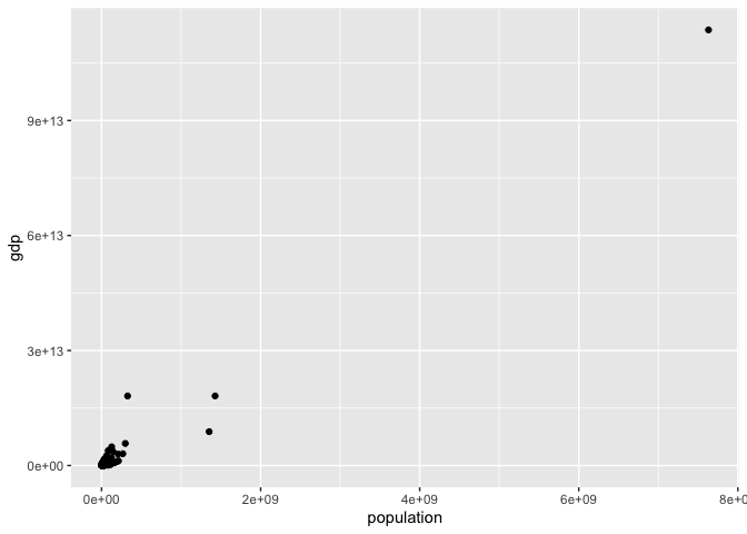
However, the plot is still rather hard to read. The scale needed to display all of the data points means that most observations in are the bottom left corner, and it is hard to see the pattern.
For data that vary over many orders of magnitude, it helps to use a log scale
ggplot( data = dat_2018,
        mapping = aes(x = population,
                      y = gdp)) +
  geom_point() +
  scale_x_continuous(trans = "log10") +
  scale_y_continuous(trans = "log10")
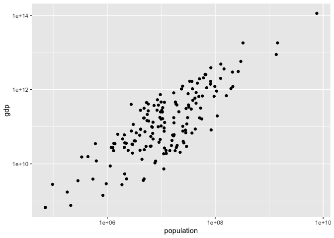
Viewed on a log scale, a linear relationship is clearly visible. Adding a linear trendline guides the eye.
ggplot( data = dat_2018,
        mapping = aes(x = population,
                      y = gdp)) +
  geom_point() +
  scale_x_continuous(trans = "log10") +
  scale_y_continuous(trans = "log10") +
  stat_smooth(method = "lm")
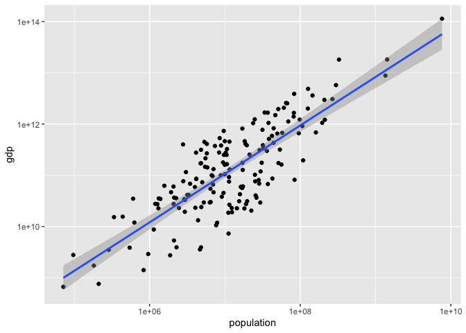
The grey interval around the trendline represents a 95% confidence interval for average GDP for a country with a given population. Note that the uncertainty is smaller in the region where there is more data, which is intuitively reasonable.
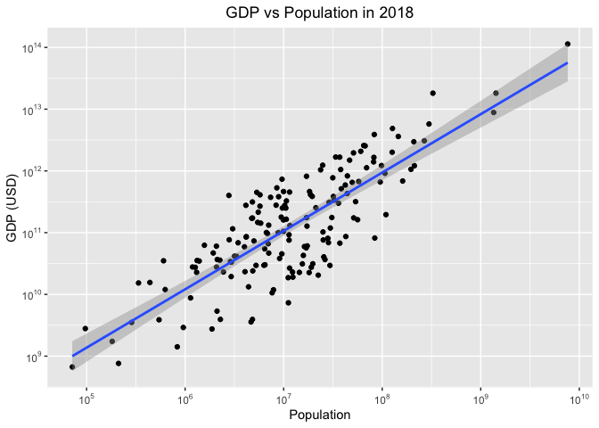
Finally, we make some cosmetic changes to the axes so that the scales
display properly. We use the breaks argument to specify where the axis
labels should be, and labels to specify the format, as powers of 10.
library(scales)
ggplot( data = dat_2018,
        mapping = aes(x = population,
                      y = gdp)) +
  geom_point() +
    scale_x_continuous("Population",
                       trans = "log10",
                       breaks = trans_breaks('log10',
                                             function(x) 10^x),
                       labels = trans_format('log10',
                                           math_format(10^.x))) +
  scale_y_continuous("GDP (USD)",
                     trans = "log10",
                     breaks = trans_breaks('log10',
                                             function(x) 10^x),
                     labels = trans_format('log10',
                                           math_format(10^.x))) +
  stat_smooth(method = "lm") +
  ggtitle( "GDP vs Population in 2018") +
  theme(plot.title = element_text(hjust = 0.5))
Next steps
In this tutorial, we have seen how to take some first steps in exploring data. In the next tutorial, you will see how to
- fit regression models in R.
- interpret linear models in context.
- understand the uncertainty in model predictions.